|
| |
nextnano3 - Tutorial
2D Tutorial
Fock-Darwin states of a 2D parabolic potential in a magnetic field
Author:
Stefan Birner.
==> This is the old website:
A new version of this tutorial can be found
here.
 -> 2DGaAs_BiParabolicQW_4meV_GovernalePRB1998.in

 -> 2DGaAs_BiParabolicQW_3meV_FockDarwin.in
Fock-Darwin states of a 2D parabolic potential in a magnetic field
In this tutorial we study the electron energy levels of a two-dimensional
parabolic confinement potential
that is subject to a magnetic field.
Such a potential can be constructed by surrounding GaAs with an AlxGa1-xAs
alloy that has a parabolic alloy profile in the (x,y) plane.
- The motion in the z direction is not influenced by the magnetic field and
is thus that of a free particle with energies and wave functions given by:
Ez = hbar2 kz2
/ (2 m*)
psi(z) = exp (+- i kz z)
For that reason, we do not include the z direction into our simulation
domain, and thus only simulate in the (x,y) plane (two-dimensional
simulation).
2D parabolic confinement with hbarw0 = 4 meV
-> 2DGaAs_BiParabolicQW_4meV_GovernalePRB1998.in
First, we want to benchmark the nextnano³ code to some other numerical
calculation:
This input file aims to reproduce the figures 1, 2, 3 and 4 of
M. Governale, C. Ungarelli
Gauge-invariant grid discretization of the Schrödinger
equation
Phys. Rev. B 58 (12), 7816 (1998).
- The GaAs sample extends in the x and y directions (i.e. this is a
two-dimensional simulation) and has the size of 240 nm x 240 nm.
At the domain boundaries we employ Dirichlet boundary conditions to the
Schrödinger equation, i.e. infinite barriers.
The grid is chosen to be rectangular with a grid spacing of 2.4 nm, in
agreement with Governale's paper.
- The magnetic field is oriented along the z direction, i.e. it it
perpendicular to the simulation plane which is oriented in the (x,y) plane).
We calculate the eigenstates for different magnetic field strengths (1 T, 2 T,
..., 20 T), i.e. we make use of the magnetic field sweep.
  $magnetic-field
   magnetic-field-on
  = yes
   magnetic-field-strength
  = 0.0d0   !
1 Tesla = 1 Vs/m2
   magnetic-field-direction
  = 0 0 1   !
   magnetic-field-sweep-active
  = yes     !
   magnetic-field-sweep-step-size
  = 0.5d0   !
   magnetic-field-sweep-number-of-steps =
  40
  !
$end_magnetic-field
- A useful quantitiy is the magnetic length (or Landau magnetic length)
which is defined as:
lB = [hbar /
(me* wc)]1/2
= [hbar / (|e| B)]1/2
It is independent of the mass of the particle and depends only on the magnetic
field strength:
- 1 T: 25.6556 nm
- 2 T:
18.1413 nm
- 3 T: 14.8123 nm
- ...
- 20 T: 5.7368 nm
- The electron effective mass in GaAs is me* = 0.067 m0.
We assume this value for the effective mass in the whole region (i.e. also
inside the AlGaAs alloy).
Another useful quantity is the cyclotron frequency:
wc
= |e| B / me*
Thus for the electrons in GaAs, it holds for the different magnetic field
strengths:
- 1 T: hbarwc = 1.7279 meV
- 2 T: hbarwc = 3.4558 meV
- 3 T: hbarwc = 5.1836 meV
- ...
- 20 T: hbarwc = 34.5575 meV
- The two-dimensional parabolic confinement (conduction band edge
confinement) is chosen so that the electron ground state has the following
energy: E1 = hbarw0 = 4 meV
(without magnetic field)
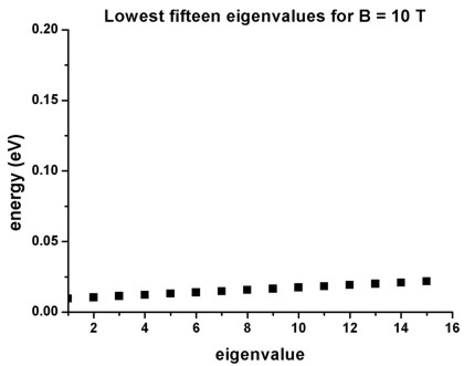
- The following figure shows the lowest fifteen eigenvalues for a magnetic
field magnitude of B = 10 T. It is in perfect agreement with Fig. 1 of
Governale's paper. The ground state has the energy E1 = 9.44 meV
(at B = 10 T).
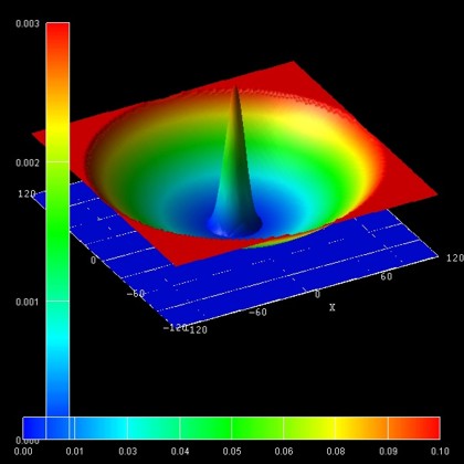
- The following figure shows the ground state probability density (psi2)
for a magnetic field magnitude of B = 10 T. It is in perfect agreement with
Fig. 2(a) of Governale's paper.
The ground state has the energy E1 = 9.44 meV (at B = 10 T).
The left, vertical axis shows psi2 in units of nm-2 (the
peak value is 0.00267 nm-2).
The parabolic conduction band edge confinement potential is also shown.
The horizontal axis shows the colormap of the conduction band edge values. In
the middle of the sample the conduction band edge is 0 eV, and at the boundary
region, the conduction band edge has the value 1.0092 eV.
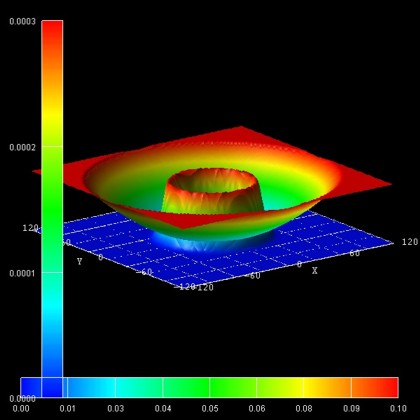
- The following figure shows the probability density (psi2) of
the 14th excited state (i.e. E15) for a magnetic field magnitude of
B = 10 T. It is in perfect agreement with Fig. 3(a) of Governale's paper.
Its energy is E15 = 21.72 meV (at B = 10 T).
The left, vertical axis shows psi2 in units of nm-2 (the
peak value is 0.000284 nm-2).
The parabolic conduction band edge confinement potential is also shown.
The horizontal axis shows the colormap of the conduction band edge values. In
the middle of the sample the conduction band edge is 0 eV, and at the boundary
region, the conduction band edge has the value 1.0092 eV.
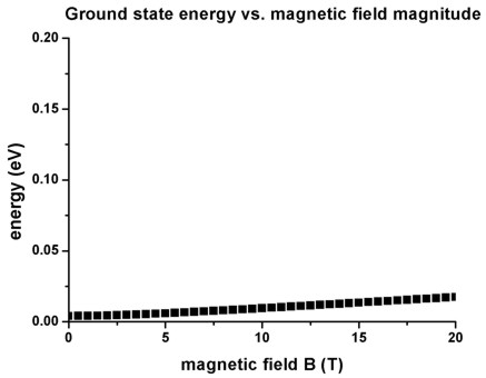
- The following figure shows the ground state energy as a function of
magnetic field magnitude. It is in perfect agreement with Fig. 4 of
Governale's paper. The ground state has the energy E1 = 4.01 meV at
B = 0 T.
2D parabolic confinement with hbarw0 = 3 meV -
Fock-Darwin spectrum
-> 2DGaAs_BiParabolicQW_3meV_FockDarwin.in
Here, we calculate the single-particle states of a two-dimensional harmonic
oscillator.
The eigenvalues for such a system are given by
En,l = (2n + |l| - 1) hbarw0
for n = 1,2,3,... and l =
0,+-1,+-2,...
(n = radial quantum number, l = angular momentum quantum number, w0 =
oscillator frequency)
The degeneracy of the eigenvalues is as follows (neglecting spin, for zero
magnetic field):
- the ground state is not
degenerate
- the second state is two-fold degenerate
- the third state is three-fold degenerate
- the forth state is four-fold
degenerate
- ...
Magnetic field
This input file aims to reproduce the Figs. 5(a) and 6(a) (which are analytical
results) of
L.P. Kouwenhoven, D.G. Austing, S. Tarucha
Few-electron quantum dots
Rep. Prog. Phys. 64, 701 (2001).
- We chose the parabolic confinement such that hbarw0
= 3 meV in agreement to this paper.
The electron effective mass is taken to be me* = 0.067 m0
(GaAs).
- The eigenvalues of a two-dimensional parabolic potential that is subject
to a magnetic field can be solved analytically. The spectrum of the resulting
eigenstates is known as the Fock-Darwin states (1928):
En,l = (2n + |l| + 1) hbar
[w02 + 1/4 wc2]1/2
- 1/2 l hbarwc for
n = 0,1,2,3,... and l = 0,+-1,+-2,...
(Note that the last term is wc and not w0
as in Kouwenhoven's paper.)
(wc = |e| B / me* = cyclotron
frequency, for GaAs: hbarwc = 1.728 meV at 1 T)
Each of these states is two-fold spin-degenerate. A magnetic field lifts this
degeneracy (Zeeman splitting). However, this effect is not taking into account
in this tutorial.
- The following figure shows the calculated Fock-Darwin spectrum, i.e. the
eigenstates as a function of magnetic field magnitude:
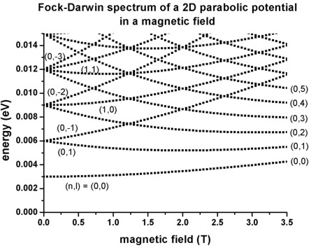
The figure is in excellent agreement with Fig. 5(a) of Kouwenhoven's paper.
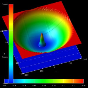
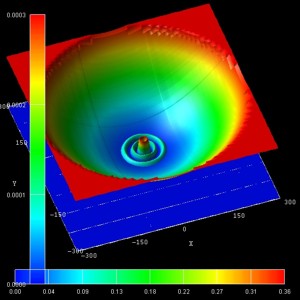
- The following figure show the probability densities (psi2) of
some of these eigenstates for a magnetic field of B = 0.05 T.
The figures are in excellent agreement with Fig. 6(a) of Kouwenhoven's paper.
The parabolic conduction band edges are also shown.
 |
 |
 |
| (n,l) = (0,0) (1st) |
(n,l) = (0,1)
(2nd) |
(n,l) = (0,2)
(4th) |
|
|
|
 |
 |
 |
| (n,l) = (1,0)
(5th) |
(n,l) = (2,0) (13th) |
(n,l) = (2,2)
(18th) |
'
- For very high magnetic fields, eventually all states become degenerate
Landau levels as can be seen in this figure. The reason is that the electrons
are confined only by the magnetic field and not any longer by the parabolic
conduction band edge.
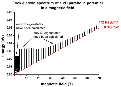
The red line shows the fan of the lowest
Landau level at 1/2 hbarwc. The higher lying states (not
shown) will collect in the second, third, ..., and higher Landau fans (not
shown).
The left part of the figure (black region) contains exactly the same
Fock-Darwin spectrum that has been shown in the figure further above (from 0 T
to 3.5 T).
|