www.nextnano.com/documentation/tools/nextnano3/tutorials/1D_TightBinding_graphene.html
nextnano3 - Tutorial
next generation 3D nano device simulator
1D Tutorial
Tight-binding band structure of graphene
Author:
Stefan Birner,
Reinhard
Scholz
If you are interested in the input files that are used within this tutorial, please
submit a support ticket.
-> 1D_TightBinding_graphene.in
Tight-binding band structure of graphene
Nearest-neighbor tight-binding approximation
In this tutorial we calculate the bulk band structure of graphene which is a
two-dimensional crystal (i.e. a monolayer of graphite) using a standard
tight-binding approach.
For more details, see for example the article
Optical Properties and Raman Spectroscopy of Carbon Nanotubes
R. Saito, H. Kataura
in
Carbon Nanotubes - Synthesis, Structure, Properties, and Applications
M.S. Dresselhaus, G. Dresselhaus, P. Avouris (Eds.)
Topics in Applied Physics, Vol. 80, Springer (2001)
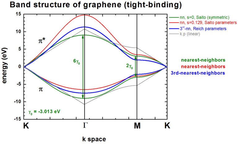
The following figure shows the conduction band pi* (upper part) and valence
band pi (lower part) of graphene along special high-symmetry directions in the two-dimensional
hexagonal Brillouin zone (k space).
The high symmetry points that are used in this graph (from left to right)
are:
- K: k = (kx,ky)
= ( 0 , 2/3 ) 2 pi/a
- Gamma: k = (kx,ky) = ( 0
, 0 )
- M: k = (kx,ky)
= ( 1/31/2 , 0 ) 2 pi/a
- K': k = (kx,ky)
= ( 1/31/2 , 1/3 ) 2 pi/a
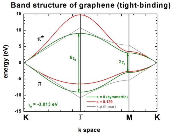
Two lines correspond to the case where the s0 parameter is set to
zero, i.e. in that case the dispersion of both pi* and pi is the same (apart
from the sign, i.e. they are symmetric with respect to the Fermi level EF
= 0 eV). In this case the splitting energy at Gamma is three times as large as
at the M point:
- splitting at Gamma: 6 gamma0
(for s0 = 0)
- splitting at M:
2 gamma0 (for s0 = 0)
Two lines correspond to the case where s0 = 0.129. pi* and pi are
then nonsymmetric and are close to calculations from first principles and
experimental data.
The data points are contained in this file:
TightBinding/BandStructureGraphene.dat
The first column contains integers which refer to the x axis (i.e.
numbering of k points), the second column contains the eigenvalue of pi* in
units of [eV] (conduction band), the third column contains the
eigenvalue of pi in units of [eV] (valence band).
The file TightBinding/k_vectors.dat contains information about which
integer corresponds to which kx and ky value.
The general formula for these lines read:
E+,- = [ E2p -+ gamma0
w(k) ] / [ 1 -+ s0 w(k) ]
The parameters can be specified in the input file:
$numeric-control

    ...
(nearest-neighbor approximation, i.e. 3
parameters)
    tight-binding-parameters =  0.0
 ! [eV]
-3.013 ! [eV] gamma0: C-C
transfer energy (usually it holds: -3 eV < gamma0
< -2.5 eV)
0.129 ! [] s0
= 0.129: denotes the overlap of the electronic wave function on adjacent sites
! 0.0 ! []
s0 = 0: denotes the
overlap of the electronic wave function on adjacent sites
!
(usually it holds: s0 < 0.1. Since this value is small, very
often, it is neglected.)
Then there are two lines that are linear around the K point (k.p
approximation or linear expansion). Their linear dispersion is independent of
the parameter s0. Thus for small values of k (i.e. with respect to
the K point), the energy dispersion
can be approximated by a linear dispersion relation.
E(k) = E2p +- hbar vF |
k | = E2p +- 31/2 gamma0 k
a / 2
where a is the lattice constant of graphene (a = 0.24612 nm) and
the Fermi velocity of the charge carriers is given by vF = 31/2
| gamma0
|
a / (2 hbar) ~= 0.98 * 106 m/s ~= 0.003 c
where c is the velocity of light.
These data points are contained in this file:
TightBinding/BandStructureGraphene_kp.dat
At the K point, the band gap is zero.
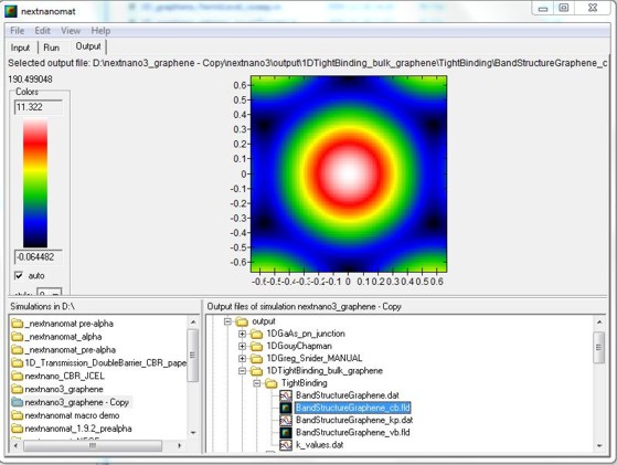
The following figure shows the energy dispersion E(kx,ky)
of graphene for s0 = 0.129.
At the K points, the band gap is zero.
The point in the middle is the Gamma point.
kx is from [-2/3,2/3] 2 pi/a, the same holds for ky.
These data points are contained in the files:
- TightBinding/BandStructureGraphene_cb.vtr

- TightBinding/BandStructureGraphene_vb.vtr
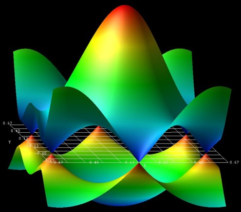
The figure has been generated using the AVS/Express software.
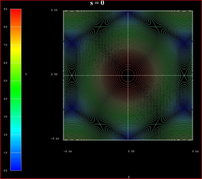
The following figure shows the contour plot of the energy dispersion E(kx,ky)
of graphene for s0 = 0 for the conduction band.
(Note that the valence band dispersion is identical, apart from the sign, for s0
= 0.)
These data points are contained in the file:
TightBinding/BandStructureGraphene_cb.vtr
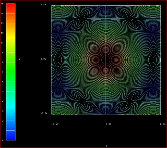
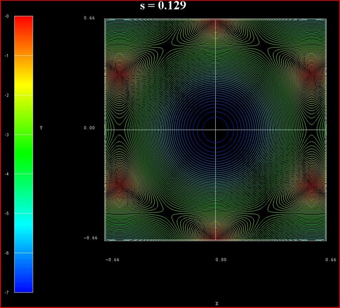
The following figure shows the contour plot of the energy dispersion E(kx,ky)
of graphene for s0 = 0.129 for the conduction band.
These data points are contained in the file:
TightBinding/BandStructureGraphene_cb.vtr
The following figure shows the contour plot of the energy dispersion E(kx,ky)
of graphene for s0 = 0.129 for the valence band.
These data points are contained in the file:
TightBinding/BandStructureGraphene_vb.vtr
nextnanomat screenshot for the conduction band dispersion E(kx,ky).
The six dark areas correspong to the Dirac points in graphene.
Output options
!---------------------------------------------------------------------------!

$output-kp-data

 ...

 bulk-kp-dispersion-3D = yes  !
In
this case, this refers to the bulk 2D tight-binding energy dispersion E(kx,ky).
!
yes, then the two-dimensional energy
dispersion E(kx,ky) is written out.
$tighten

 destination-directory = TightBinding/

 !-------------------------------------------------------------------------!

 ! This parameter defines the resolution of the E(kx,ky) energy
dispersion.

 ! E.g. if 'number-of-k-points = 100' then
the kx gridding has a total of

 ! [-100,...,0,...,100] grid points,

 ! i.e. a total of 2 * 100 + 1 = 201 grid points along the kx direction.

 ! The same applies for ky direction.

 !-------------------------------------------------------------------------!

 number-of-k-points = 100
! ==> 2 * n + 1
Third-nearest-neighbor tight-binding approximation
The following figure shows the band structure of graphene.
All lines are identical to the ones shown already above with the exception of
the blue lines which is the third-nearest-neighbor tight-binding approximation.
The third-nearest-neighbor tight-binding approximation is described in the
following paper:
[Reich]
Tight-binding description of graphene
S. Reich, J. Maultzsch, C. Thomsen, P. Ordejon
Physical Review B 66, 035412 (2002)
The following parameters have been used:
(third-nearest-neighbor approximation,
i.e. 7 parameters)
    tight-binding-parameters = -0.28
 ! [eV]
-2.97 ! [eV] gamma0: C-C
transfer energy (nearest-neighbor, nn)
0.073 ! [] s0:
denotes the overlap of the electronic wave function on adjacent sites (nn)
-0.073 ! [eV] gamma1: (2nd-nn)
0.018 ! [] s1:
(2nd-nn)
-0.33 ! [eV] gamma2: (3rd-nn)
0.026 ! [] s2:
(3rd-nn)
(The parameters are taken from Reich et al. Note
that the band gap at the K point is not exactly zero when using these
parameters.)
More options...
Inside the code several options, i.e. several algorihms, exist to setup the
tight-binding Hamiltonian:
tight-binding-method = bulk-graphene-Saito-nn
!     nn =
nearest-neighbor
= bulk-graphene-Scholz-nn      !
    nn =
= bulk-graphene-Scholz-3rd-nn  !
3rd-nn =
= bulk-graphene-Reich-3rd-nn   !
3rd-nn =
Special option for third-nearest-neighbor tight-binding approximation in
graphene:
tight-binding-calculate-parameter = no
 !
(default) use 7
parameters (E2p,gamma0,gamma1,gamma2,s0,s1,s2)
= E2p !
= gamma1 !
E2p or gamma1 can be calculated internally in order to
force E(K) = 0 eV where K is the K point in the Brillouin zone. In that case,
only 6 parameters are used (although 7 parameters have to be present in the
input file). The parameter to be calculated is simply ignored inside the code.
The k space resolution, i.e. the number of grid points on the axis of these
plots can be adjusted.
  $tighten

   calculate-tight-binding-tighten = no
!

   destination-directory
= TightBinding/

   number-of-k-points
= 50
!
This corresponds to 50 k
points between the Gamma point and the M point.
!
|